The Median of Classified Data
Definition
Recall that the definition of the median is different for odd and for even numbers of observations when the data are not classified. However, if the n data are classified, then it is simply defined as “n/2” observation. Thus, if we have the frequency distribution of 100 observations, then the 50th observation in order of size would be the median. If we have 101 observations then the 50.5 observation would be the median. If the reader is puzzled by what the phrase the 50.5 observation means, we will be in a better position to explain this phrase after the following example.
Explanation with example
Consider the frequency distribution shown in Table below.
| Class | Class boundaries | Frequencies |
| 1 | 49-5- 995 | 17 |
| 2 | 995—149-5 | 38 |
| 3 | 149-5—199-5 | 61 |
| 4 | 199-5—249-5 | 73 |
| 5 | 249-5-299-5 | 56 |
| 6 | 2995—349-5 | 29 |
| 7 | 349-5—399-5 | 16 |
| 8 | 399-5—4495 | 10 |
| 300 |
The median of this frequency distribution is the 150th observation. There are 116 observations in the first three classes, and 189 in the first four. The 150th observation is in the fourth class, which, since it contains the median, is called the median class. We know that the median lies in the interval from 199.5 to 249.5, but we don’t know exactly where. We can make an estimate (an educated guess) of the median by linear interpolation if we assume that the observations are distributed uniformly throughout the interval from 199.5 to 249.5.
Distributed Uniformly
The term ‘distributed uniformly’ means the following. If one thinks of the interval from 199.5 to 249.5 as being marked off on a scale it would be 50 units long. If the 73 observations which the class contains are distributed uniformly throughout the interval there would be an observation every of a unit. In other words, if the 50 units comprising the interval were divided into 73 equal intervals, then each interval would contain one observation.
Example
To find it, we must count 34 observations into the fourth class because the median is the 150th observation and the first three classes contain only 116 observations. Hence, it is located at the point which is of the distance along the fourth class interval. This point is 34/73 . (50) units to the right of 199.5, the lower boundary of the fourth class. Thus, the median equals
199.5 + 34/73 . (50) = 199.5 + 23.3 = 222.8
General Formula for finding the median
We can reason in exactly the same manner to obtain a general formula for finding the median value for classified data.
First, we need to find the class which contains the middle observation. Let M denote the number of this class. Where M is some integer from 1 to k. If the median occurs in the fifth class, then M=5. If it occurs in the seventh class, then M=7 and so on.
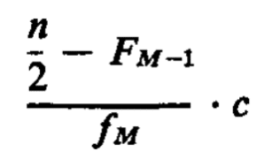
Let the frequency of the M th class be denoted by Fm. Next, note how many observations are in the M — 1 classes preceding the median class. Denote this cumulative frequency by Fm—1.
The number of observations which we must count into the median class in order to find the median equals the difference between n/2. The number of the middle observation, and the number of observations in the classes below the median class. Using the symbolism introduced in the preceding paragraph, this difference is n/2 — Fm—1.
There are fm observations in the median class and assuming that the observations are distributed evenly throughout the median class.
The value of it is as follow of the distance along the class interval. 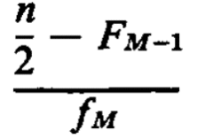
Hence, we see that the general formula for the middle of classified data is as follow.
Where,
bL = lower boundary of the median class.
n = number of observations.
fm = the number of observations in the median class.
fm—1 = the number of observations in the M — 1 classes preceding the median class.
Explanation through example
In the above example on Table we had
bL = 199.5
n = 300
fm—1 = 116
fm = 73
c = 50
So that
M = 199.5 + (150 — 116) \ 73 . 50 as already indicated.
Now it should be clear why it is defined as the n/2 th observation, regardless of whether n is odd or even.
Recall that in a histogram the areas of the rectangles are proportional to the numbers of observations in each of the respective classes. Thus, a vertical line through the median should divide the histogram into two parts of equal areas. This is consistent with the previous definition. That the number of observations on one side of the median equals the number of observations on the other. Because the areas here are analogous to the observations in the previous definition of the median.
If we had a sample of 101 classified observations, and if we said that the median is the 51’st observation we would need to find the point where the 51’st observation is estimated to be. At this point an area corresponding to 51 observations is to the left. And to the right is an area corresponding to only 50 observations. Since the areas are unequal, this point is not the median. If, on the other hand, we take the 50.5th observation to be the median. Then the point where this observation is estimated to be will exactly divide the histogram into two parts of equal areas—an area corresponding to 50.5 observations lies to its left. And an area corresponding to 50.5 observations lies to its right.
Relation between Measures of Location and the Types of Frequency Curves for the median, mode and mean
In practice, the frequency curves have the following shapes given below.
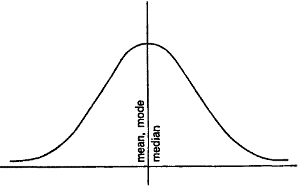
Fig. 1 shows a symmetrical curve in which the mode, median, and mean coincide.
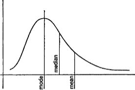
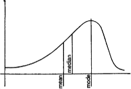
Fig. 2 and Fig. 3 show two skew frequency curves and the relative positions of the measures of location.
Notice that each one of the above curves is unimodal.


