The Mode, Median and Arithmetic mean

The Mode

Definition of the mode

The mode is defined as the observation in the sample which occurs most frequently, if there is such an observation. If each observation occurs the same number of times, then there is no mode. If two or more observations occur the same number of times. And more frequently than any of the other observations then there is more than one mode. The sample is said to be multi-modal. If there is only one mode the sample is said to be unimodal.

Examples of the mode

1.  If the sample is 14, 19, 16, 21, 18, 19, 24, l5, 19, then the mode is 19.
2. If the sample is 6, 7, 7, 3, 8, 5, 3, 9, then there are two modes, 3 and 7 [bimodal].
3. If the sample is 14, 16, 21, 19, 18, 24, 17, then there is no mode.

The Median

Definition of the median

If the sample observations are arranged in order from smallest to largest, the median is defined as the middle observation. If the number of observations is odd, and as the number half-way between the two middle observations if the number of observations is even.

The median Examples

1. Given the sample 34, 29, 26, 37, 31. Arranged in order we have 26, 29, 31, 34, and 37. The number of observations is Odda and therefore the median is 31.
2. Given the sample 34, 29, 26, 37, 31, 34. Arranged in order we have 26, 29, 31, 34, 34, 37. The number of observations is even. The median is half-way between the third and fourth (the two middle)observations. Thus the median is 32.5.

The Arithmetic Mean

Definition of the arithmetic mean

The most commonly used measure of location is the arithmetic mean, called simply the mean.

The definition is simple:

Sample mean = Sum of the observations / Number of observations

The number of observations is usually denoted by n.

Also, the first (not in order of size, but simply in the order examined or written) observation is denoted X1 (read ‘X sub one’ or merely ‘X one’).

The second observation is denoted X2.

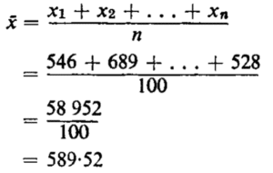
The third is denoted X3, and so on until the last observation, denoted Xn. The mean of the sample is denoted by the symbol X (read ‘X bar’). Thus the definition above can be written as

where the symbolism … + Xn» means that we are to continue adding the observations until we reach the last one which is Xn.

Example 1

If our sample consists of the data 8, 7, 11, 8, 12, 14, then the mean is

X bar = 8 + 7 + 11 + 8 + 12 + 14 / 6

= 60 / 6

= 10

 Note that, as the sample observations are written above, X1 = 8, X2 = 7, X3= 11, X4 = 8, and so on.

EXAMPLE 2

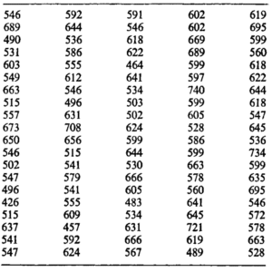
Consider the SAT—Verbal data. From Table given below:

we have

In summary, we have found four different values for the ‘centre’ of the SAT—Verbal data by using four different measures of location.

1. Mid-range equals 583.
2. The mode equals 599.
3. Median equals 598.
4. The mean equals 589.52.

To briefly compare the four measures of location discussed we make the following observations.

Mid Range

The mid-range is easy to find, but because only two observations are involved in the définition it neglects most of the information which is present in the entire sample.

The Mode

The mode is a satisfactory measure of location if the frequency distribution of the sample is rather symmetrical. But if the frequency distribution is not symmetrical the most frequent observation might be far removed from the ‘centre’ of the sample. The mode would not be a very good measure of location.

Median

The median has much to commend it. Its definition makes use of all observations. Extreme observations do not cause the median to fluctuate much. For instance, the median of 13, 14, 16, 18, 21 is 16 and the median of 13, 14, 16, 18, 21, 50 is 17. The 50, which is much larger than any of the other observations, causes very little change in the median. The median is very easy to find when the data have been arranged in order. Another advantage of the median occurs in situations when data are classified and there is an open class. For instance, if the class intervals of a frequency distribution are 100 but not 200, 200 but not 300, 300 but not 400, 400 or more, then it is impossible to calculate the mean—because the open class, ‘400 or more’, has no upper boundary.

Mean

This is not true for the mean, because the mean of 13, 14, 16, 18, 21 is 16-4 and the mean of 13, 14, 16, 18, 21, 50 is 22. We have a change of about 34 per cent in the mean, which is about six times the change in the median.

One of the primary advantages of the mean as a measure of location is that if we have a mean for each of several samples and want to find the mean of the sample which results when the several samples are combined this can be easily done. If the medians of several samples are known and the median of the combined samples is desired, it cannot be found as quickly as the mean. When tests of hypothèses are made about the ‘location’ of the population, tests about the mean are more powerful than tests about the median, although somewhat more restrictive assumptions need to be made. Another advantage of using the mean is that the data do not have to be arranged in order, as they do when the median is used.